Data editing


You can modify any data plotted with plt, either one point at a time or over a specified range. If your data was plotted as an intensity map using the image pseudo object, use the methods described in the second section below (3d data editing). Otherwise, use the methods described in the first section (2d data editing).

2d data editing

There are three methods of 2d data editing, each with different advantages.

The first method is to use the Cursor Data Window which is the best method when you want to make many edits to several different traces. The strength of this method is that you can see the results of the changes for many points and many different traces at the same time as well as its multi-level undo/redo capability. Its only weakness is that you can't drag points to new locations with the mouse (i.e. it is only keyboard-driven). How to use the Cursor Data Window is explained in detail in the Menu box section here.

The second method is to use the built-in line property editor. This method is conceptually the simplest but is only practical for making minor data changes to lines containing just a few points.


To start the line property editor, first click on the line you want to edit, then RIGHT click on the Ycursor edit box. (This is the edit box closest to the lower right corner of the figure.) This will open the popup menu you see here.

Then choose the first selection from this popup (Properties) to open the properties editor.

Next, click on the popup menu under the Line properties heading. As shown here, this will give you a choice of line properties. Then click on "Xdata", "Ydata", or "Zdata" depending on which coordinate you would like to modify. Then the X,Y, or Z line data (whichever you chose) will appear in the edit box below the popup. Since the edit box is small, you will only be able to see the first two or three values, but you can use the left/right keys to scroll to the data element you want to change. Then you can use the usual keyboard entry methods to enter the new value or values you want, which will be accepted when you press the enter key. You can't add or remove points using this method, i.e. you can only edit points that are already there. (As I mentioned before ... simple, but primitive).

The bottom popup menu of the properties editor is used to modify other miscillaneous figure properties as described here.

The third method of 2D data editing is the graphical method, which primarily depends on using the mouse to move, add, or remove data points. (This method allows keyboard entry as well, but you probably won't use that method often.) As before, the first step is to click on the trace containing the data you want to edit, followed by a right click on the Ycursor edit box which again brings up the popup shown below.


Above, we have already discussed the first menu (the Properties editor).

The next two choices (unrelated to data editing) are multiCursor which toggles the multiCursor mode (described here in the Cursoring section) followed by xView slider which toggles the xView slider (described in the here in the Zooming and panning section).

The fourth menu choice (Undo) will reverse the previous edit operation that was done using the remaining options in this popup. If the previous operation was a range edit (described below) then all the data points within the selected range will revert to their previous value. This is a single-level undo (i.e. you can't undo multiple edit operations). If no edits have been made, the Undo selection will have no effect other than reverting the edit cursor (if it's enabled) back to the standard cursor shape.

The remaining six selections in this popup contain the actual data editing commands. The descriptions below are written for completeness rather than brevity so don't be scared off. The commands are intuitive, so you may be better off skipping the descriptions at first in favor of experimentation. The six editing commands are divided into these two types:

Modify
The modify commands change the x or y coordinates (or both) of a single data point by moving the edit cursor with the mouse. After a modify command, the lengths of the x and y vectors normally don't change ... however, there are two exceptions to this. The first is called the "delete mode" which is activated by dragging the edit cursor to any point outside the axis boundary. The point dragged will be removed causing the lengths of the x and y vectors to decrease by one. The 2nd exception is called the "insert mode". The insert mode is activated by dragging the edit cursor with the right mouse button instead of the usual left button. With the insert mode, the lengths of the x and y vectors will both increase by one.
Range
With the range commands the length of the x and y vectors remain the same. The range commands allow you to modify many consecutive data elements at once. All the data points between the current cursor location and the location modified during the previous data editing command are modified so that all these points lie on a straight line connecting the two end locations. For this to work, the previously edited point and the current cursor location must both lie on the same line. If this is not true, then the Range commands behave just like the Modify commands described above. You can recognize whether the range operation or the modify operation is in progress based on the shape of the edit cursor (See cursor shapes table below).

The six commands are also split into three categories which are identified by the arrows next to each command as follows:


Modify↑↓
Range↑↓
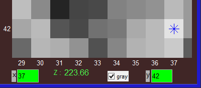
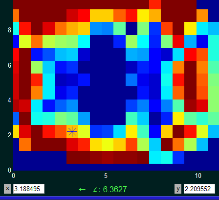
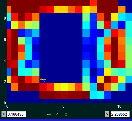
These are perhaps the two most commonly used of the data editing menus. As soon as you select the editing mode, the regular data cursor disappears and is replaced by an editing cursor with a different shape. (See data editing cursor shapes below). Then you can grab the edit cursor with the mouse and drag it to the desired location. However, you will only be able to move the cursor up and down (i.e. only the y coordinate is allowed to change). This is useful because in many data sets, the independent variable (x) represents a specifically chosen set that you want to keep fixed. As soon as you release the mouse button (after dragging the edit cursor to its new location) the edit command will take effect, the edit cursor will disappear, and the normal data cursor will reappear. The cursor then reverts to its usual data exploration function, and to edit another data point you must right click yet again on the Ycursor edit box and select the desired data edit operation. This back-and-forth operation (which I will call the "normal editing mode" is convenient when you just have a few data points to modify, but can become cumbersome when you want to edit many data points in succession.

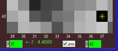
In that situation, you can switch to "persistent editing mode". (The persistent editing mode applies only to the three Modify selections and does not apply to any of the Range selections). To enable the persistent editing mode for Modify up/down, bring up the data editing menu as usual, but then instead of left clicking on the Modify up/down selection, click on it with the right mouse button. The label in front of the Ycursor edit box (gray) normally contains the letter "y" (as shown to the left) but this label will switch to the delta symbol (also shown to the left) which indicates that you are now in persistent editing mode. Once in this persistent mode, you can continue to modify as many points on the graph as you want (including insert and delete operations) without having to open the data editing menu each time. The only drawback is that you have to forgo the usual data exploration features of the cursor, however, you can restore the default mode by double RIGHT clicking on the Ycursor edit box (at which point the Ycursor label changes from the delta back to the "y").

Modify↔
Range↔
These two menu options behave identically to the two commands described above except for the fact that with the mouse you can only drag the cursor left or right (i.e. only the x coordinate is allowed to change). It is far more common to want to change the y coordinate (using the selections above) or to use the selections below to have the freedom to move the point anywhere (modifying both coordinates), however, the left/right option is included for completeness. You can also select this option with the persistent editing mode by right clicking on the Modify left/right option. The gray "y" label of the Ycursor editbox changes to a ">" greater than sign (as shown at the left) to indicate the persistent mode is enabled. Again, you can restore the normal editing mode by double RIGHT clicking on the Ycursor edit box, which will cause the label to revert to "y" indicating the normal editing mode.

  Modify  
  Range  
When using these last two menu options you can use the mouse to drag the edit cursor anywhere (i.e. you can change both the x and y coordinates of the point. You can select this option with the persistent editing mode by right clicking on the Modify option. The gray "y" label of the Ycursor editbox changes to a solid diamond symbol (as shown at the left) to indicate the persistent mode is enabled. Again, you can restore the normal editing mode by double RIGHT clicking on the Ycursor edit box, which will cause the label to revert to "y" indicating the normal editing mode.

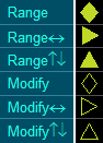
The usual data cursor is a plus sign or a small circle, but once you select one of the six editing modes, the data cursor changes to one of the six edit cursors shown in this table. (Although a single edit cursor shape would suffice, these six cursor shapes make it clear which editing mode you are using.)

Whenever you see one of these six data cursors, in addition to dragging the cursor with the mouse, you also have the opportunity to type a new x or y value into the x or y cursor edit boxes. This allows you to enter values more precisely than what is possible with a mouse movement. In all six modes, you may enter a new value in either the x or y edit boxes. (So, for example with the Modify up/down selection, you can still type in a new value into the x edit box, thus bypassing the "y-only" restriction of the mouse movement.) With the ↑↓ and ↔ editing modes, data editing is terminated as soon as you type a value into the x or y edit box. However, for the unrestricted modes, (i.e. Modify or Range without the arrows) data editing isn't terminated until you click on one of the data traces with the mouse. This allows you to enter both x and y values as well as to experiment with different entries before accepting any particular value.

When dragging a data edit cursor around, plt attempts to limit the allowed positions so that the x and y values can be represented in as few digits as possible while still allowing the cursor to be positioned at every pixel in the axis. If you find that you are not able to position the edit cursor at the exact desired spot, you can increase the number of possible positions by increasing the size of the figure, or by zooming the axis in the vicinity of the edit cursor. Another strategy is to simply type the desired value for the x and/or y positions of the edit cursor into the respective edit boxes as described in the previous paragraph. On the other side of the spectrum, sometimes you may want to further limit the allowable positions of the edit cursor to make it easy to place it at cardinal points. You can do this by typing a complex number into the Y edit box.

For example, if you enter the number 20i into the Y edit box, the allowed positions as you drag the edit cursor will be approximately 20 pixels apart in both the x and y directions. This is equivalent to typing the command setappdata(ax,'eRes',[20 20]); where ax is the axis containing the edit cursor. Typing 1i into the Y edit box would return the edit cursor resolution to the default value of 1 pixel.

As another example, suppose we enter the number 3+10i into the Y edit box. This will set the x edit resolution to 3 pixels and the y edit resolution to 10 pixels which also can be accomplished by typing the command setappdata(ax,'eRes',[3 10]);. (Sometimes it is useful to have different resolutions in the x and y directions.)

Note that after typing a complex number into the Y edit box, the message "eRes set" will appear in the edit box to notify you that the new edit resolution has been accepted.

Data Editing programming features

Although programming features and techniques are generally discussed in the "Programming with plt section, the following information is included here because it relates closely with the data editing user interface features shown above.

If you don't like the default size that plt chooses for the six data edit cursors, (shown in the table above) you can change this with a command such as: setappdata(gcf,'CurEdit',14). The new size will be used the next time a cursor edit mode is selected.

If you want to prevent a line from being edited, set the line's tag property to 'NoEdit'. With that line property set, any attempt to edit that line will be ignored.

If plt was called using the MotionEdit parameter, the function specified with that parameter will be called continuously as you drag the edit cursor around. This function may be used to create or modify text, plots or other gui objects on the screen. The sig\editz.m, sig\editz.m, and demo\hermite.m programs all demonstrate the use of the MotionEdit parameter. (Also see Mouse Motion Functions)

If you want to save the altered data (to a file for example) you have to get the data from the 'xdata' and 'ydata' properties of the line handle. (Remember the line handles are returned by the plt call.) When the user modifies any data using these data editing functions, plt executes the user-specified move cursor callback. (See the description of the 'set','moveCB' function here.) The callback routine or any other part of your application can use the 'NewData' application property of the current figure window to determine if data has been modified by one of the data edit commands. For example:

index = getappdata(gcf,'NewData'); % returns the index where xdata/ydata was modified
if index                           % is there any new data?
  DataWasModifiedAction(index);    % yes, process the new data
  setappdata(gcf,'NewData',0);     % indicate that the data was already processed
end;

Note that the NewData property only gets set after a data edit operation is complete, unlike the MotionEdit function which gets called as you are dragging a cursored value to its new location. There is one additional figure application data variable called Dedit that may also be useful for an application using the data editing feature. The command getappdata(gcf,'Dedit') will return the following 9 element cell array:

'Dedit' figure application data (cell array)
1
The CursorID associated with the edited trace
2
A number from 1 to 6 which identifies which data edit command is being used (in the order that they appear in the popup):
    1:  Range
    2:  Range Left/Right
    3:  Range Up/Down
    4:  Modify
    5:  Modify Left/Right
    6:  Modify Up/Down
3
The handle of the cursor object associated with the modified data.
4,5
For internal use. (This saves the cursor marker shape and size so that the normal cursor can be restored when the data edit operation is complete.)
6
For internal use. (This saves the edited trace x/y data so that it can be restored by the undo function (right clicking on the "Cancel" option)
7,8
For internal use. (This saves the position index and trace number of the previously edited trace - information is needed for the modify range operations.)
9
The position index of the cursor into the edited trace
10
The edit cursor resolution in the horizontal direction (in pixels)
11
The edit cursor resolution in the vertical direction (in pixels)

After performing a data edit operation you will likely want to perform another data edit using the same data edit command. Thus it would be nice if you could initiate another data edit operation without having to again select one of the nine data editing operations. In fact, there is a way to do this - simply right-click on the Xcursor edit box. This behaves similarly to what happens when you right-click on the Ycursor edit box except you don't get the menu of data editing choices, since it will use your previous selection. There has to be a default for this operation in case the user right-clicks on the Xcursor edit box before doing any other data edit operation. The default is "Modify" since this is the most commonly used operation. It is rare to want to change this default, although you can do so by changing the second element of the Dedit application variable as described above.

If you create a figure with a plt command that includes the parameter 'MotionEdit','funcname', then while you are modifying a data value by using the data editing feature, the function funcname(a) will be continually called as the mouse is moved (i.e.  for as long as the mouse button is held down). The parameter "a" is a nine-element cell array containing information related to the edited trace (as described in the table above). Alternatively, you can define the MotionEdit function after the call to plt with the following command:

    setappdata(gca,'MotionEdit',{@funcHandle param1});

The application editz.m shows how the MotionEdit function can be used to reposition the plotted poles and zeros. Note that allowing the plot to be updated as the data is being edited has an impressive advantage for that application.

The hermite.m example also demonstrates the use of the MotionEdit parameter to update the polynomial interpolation of a vector field in real time.

In addition, you may also define functions that get called when a data edit operation begins or terminates. These two functions (respectively) may be defined as follows:

    setappdata(gcf,'EditStart',@StartFuncName);
    setappdata(gcf,'EditStop', @StopFuncName);

Usually, you enter one of the data editing modes by selecting one of the entries in the Yedit popup menu with the mouse, however, this can be initiated from a program as well. For example, the command plt click Yedit 6; or its functional form plt('click','Yedit',6); puts the cursor into the "modify up/down" mode, since that is the 6th selection in the menu shown above. (Note that the "6" refers to the sixth entry in the Yedit popup menu. The full list of commands similar to this is shown in the table below:

plt xleft EDIT 1; Enter data editing (using last used editing mode)
plt xleft EDIT 2; Open up Yedit popup menu
plt xleft EDIT 5; Exit data editing mode
plt xleft Yedit 4; Cancel data editing mode
plt xleft Yedit 5; Enter data edit mode (Range)
plt xleft Yedit 6; Enter data edit mode (Range left/right)
plt xleft Yedit 7; Enter data edit mode (Range up/down)
plt xleft Yedit 8; Enter data edit mode (Modify)
plt xleft Yedit 9; Enter data edit mode (Modify left/right)
plt xleft Yedit 10; Enter data edit mode (Modify up/down)
plt xright Yedit 8; Enter persistent data edit mode (Modify)
plt xright Yedit 9; Enter persistent data edit mode (Modify left/right)
plt xright Yedit 10;  Enter persistent data edit mode (Modify up/down)

3d data editing

When the data has been plotted using plt('image',...) (i.e. the image pseudo object) you can use the method described below to edit the data in the plotted intensity map. You can practice using these methods with these programs that use the image pseudo object:

Modifying a single pixel at a time


To edit a single pixel, first expand the axis so that each individual pixel near the region you want to modify is easily visible. If you don't know how to do that, review the Zooming and panning section. Next, click on the pixel that you want to edit. In this example, we have clicked on the pixel at (x,y) coordinates (37,42). The cursor marker (an asterisk symbol) will always appear in the middle of the pixel. Its current Z value (i.e. intensity) will appear below the graph after the "Z:" label. In this example (using the picplot.m demo in its grayscale mode) the Z value for this pixel is 223.66. Suppose we want to change this value to 4.4. Right click on the 223.66 number and then press the backspace key until the number is erased and then type "4.4" and press enter. (Instead of the backspace key, you could also use the down arrow key. That's harder to remember, but it's faster since you only have to press the down arrow key once to erase the entire number.)

The figure will now look like this. Notice that the chosen pixel has changed to black and the Z value readout shows the new pixel value. Also, note the cursor color has also changed. (This is because plt ensures that the contrast between the cursor and the pixel color is as high as possible.) Notice that a new symbol has appeared (a left arrow) just to the left of the Z: label. This is the undo symbol. If you now click on the undo symbol, the Z value will revert to 223.66 (the value the pixel held before editing). Since this was the only data edit we have done, the left arrow symbol will disappear indicating that there is nothing left to undo. There is essentially no limit (beyond the amount of memory allocated to Matlab) to how many undo operations are allowed. If you make 100 edits, the left arrow will remain visible until you click on it 100 times as each of the edits are reversed. Modifying the same pixel twice in a row is treated like a single edit. For example, if we modified the 4.4 value again (to say 5.5) without changing a different pixel in between) then pressing undo will not change it back to 4.4 but rather back to 223.66 (its original value).

In addition to typing the new Z values as we just described, if you want to change the intensity value more gradually you can left click just to the right or left side of the current Z value to increase or decrease the Z value by 1. You can also hold down the mouse button after clicking and the Z value will continue to increase or decrease until you release the mouse button. The pixel value will slowly change its color as you are holding down the mouse button and the cursor marker will also change as necessary to maintain adequate contrast with the surrounding pixel color.

Modifying a rectangular region


In addition to editing a single point, we can fill a rectangular region with a constant value. We start by placing the cursor on any corner of the region we would like to fill. In this example, I have chosen to cursor the upper right corner of the fill region at the (x,y) coordinates (6.377,8.102). The Z value at this point happens to be 6.3951 as you can see by the Z readout at the bottom of the figure. For this particular color map (jet) this Z value corresponds to the orange pixel you see in the cursored square. (Note: You can replicate this figure by running the pltmap.m demo program and then moving the resolution slider all the way down to its lowest setting of 25 pixels).

Next, we enter the desired fill value (zero in this example) by right clicking on the current Z value (6.3951), entering backspaces followed by a zero and then pressing enter. This is the same process described above for editing a single pixel, and indeed only the one pixel chosen has been modified as shown here.

Next, we cursor the opposite corner of the desired rectangle. In this example, I have cursored the point (3.188,2.209) which will be the lower left of the fill region. As you can see, the Z value of this point is 6.3627 (which is similar to but not identical to the original Z value of the upper right corner pixel).

To complete the fill operation, right click on the yellow Z: text string which is located at the bottom of the figure between the left arrow symbol and the zero character that indicates the fill value for the region. As soon as you do that, the selected region will be filled and the figure will look like this one. This may feel like two edit operations, but it is recorded as a single edit operation which means that clicking on the left arrow will restore the entire fill region to contain the values that it had before the rectangular fill operation began. If no other pixels were edited, the left arrow symbol will disappear indicating that there is nothing left to undo. The undo buffer may contain a mixture of single point and rectangular fill edit operations and they will be undone one item at a time (in the reverse order that they were entered) until the left arrow disappears and the plot is returned to its original configuration.